Binary Search Trees
In the introduction we used the
binary search algorithm
to find data
stored in an array. This method is very effective, as each
iteration reduced the number of items to search by one-half.
However, since data was stored in an array, insertions and
deletions were not efficient. Binary search trees store data in
nodes that are linked in a tree-like fashion. For randomly
inserted data, search time is O(lg n). Worst-case behavior
occurs when ordered data is inserted. In this case the search
time is O(n). See
Cormen [1990]
for a more detailed description.
Theory
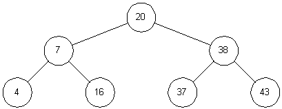
A binary search tree is a tree where each node has a left and
right child. Either child, or both children, may be missing.
Figure 3-2
illustrates a binary search tree. Assuming k
represents the value of a given node, then a binary search tree
also has the following property: all children to the left of the
node have values smaller than k, and all children to the right
of the node have values larger than k. The top of a tree is
known as the root, and the exposed nodes at the bottom are known
as leaves. In
Figure 3-2,
the root is node 20 and the leaves are
nodes 4, 16, 37, and 43. The height of a tree is the length of
the longest path from root to leaf. For this example the tree
height is 2.
To search a tree for a given value, we start at the root and
work down. For example, to search for 16, we first note that 16 < 20
and we traverse to the left child. The second comparison
finds that 16 > 7, so we traverse to the right child. On the
third comparison, we succeed.
Each comparison results in reducing the number of items to
inspect by one-half. In this respect, the algorithm is similar
to a binary search on an array. However, this is true only if
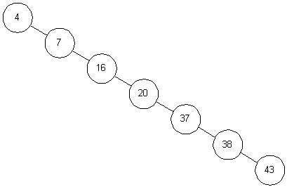
the tree is balanced. For example,
Figure 3-3
shows another tree
containing the same values. While it is a binary search tree,
its behavior is more like that of a linked list, with search time
increasing proportional to the number of elements stored.
Insertion and Deletion
Let us examine insertions in a binary search tree to determine
the conditions that can cause an unbalanced tree. To insert an
18 in the tree in
Figure 3-2,
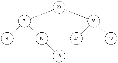
we first search for that number.
This causes us to arrive at node 16 with nowhere to go. Since 18 > 16,
we simply add node 18 to the right child of node 16
(Figure 3-4).
Now we can see how an unbalanced tree can occur. If the data
is presented in an ascending sequence, each node will be added to
the right of the previous node. This will create one long chain,
or linked list. However, if data is presented for insertion in a
random order, then a more balanced tree is possible.
Deletions are similar, but require that the binary search tree
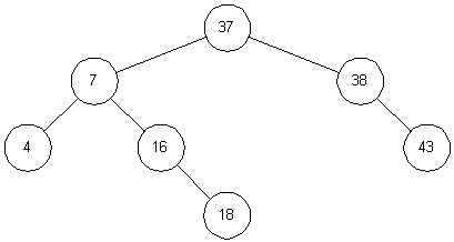
property be maintained. For example, if node 20 in
Figure 3-4
is
removed, it must be replaced by node 37. This results in the
tree shown in
Figure 3-5.
The rationale for this choice is as
follows. The successor for node 20 must be chosen such that all
nodes to the right are larger. Therefore we need to select the
smallest valued node to the right of node 20. To make the
selection, chain once to the right (node 38), and then chain to
the left until the last node is found (node 37). This is the
successor for node 20.
Implementation
An
ANSI-C implementation
for a binary search tree is included.
Typedef T and comparison operators compLT
and compEQ should be altered to reflect the data stored in the
tree. Each Node consists of left, right, and parent
pointers designating each child and the parent. Data is stored in the
data field. The tree is based at root, and is initially NULL.
Function insertNode allocates a new node and inserts it in the tree.
Function deleteNode deletes and frees a node from the tree.
Function findNode
searches the tree for a particular value.


